Recipes

Here you can find some useful snippets of code to make using ESPEI easier.

Optimal parameter TDBs

Creating TDBs of optimal parameters from a tracefile and probfile:

"""
This script updates an input TDB file with the optimal parameters from an ESPEI run.

Change the capitalized variables to your desired input and output filenames.
"""

INPUT_TDB_FILENAME = 'CU-MG_param_gen.tdb'
OUTPUT_TDB_FILENAME = 'CU-MG_opt_params.tdb'
TRACE_FILENAME = 'trace.npy'
LNPROB_FILENAME = 'lnprob.npy'

import numpy as np
from pycalphad import Database
from espei.analysis import truncate_arrays
from espei.utils import database_symbols_to_fit, optimal_parameters

trace = np.load(TRACE_FILENAME)
lnprob = np.load(LNPROB_FILENAME)
trace, lnprob = truncate_arrays(trace, lnprob)

dbf = Database(INPUT_TDB_FILENAME)
opt_params = dict(zip(database_symbols_to_fit(dbf), optimal_parameters(trace, lnprob)))
dbf.symbols.update(opt_params)
dbf.to_file(OUTPUT_TDB_FILENAME)

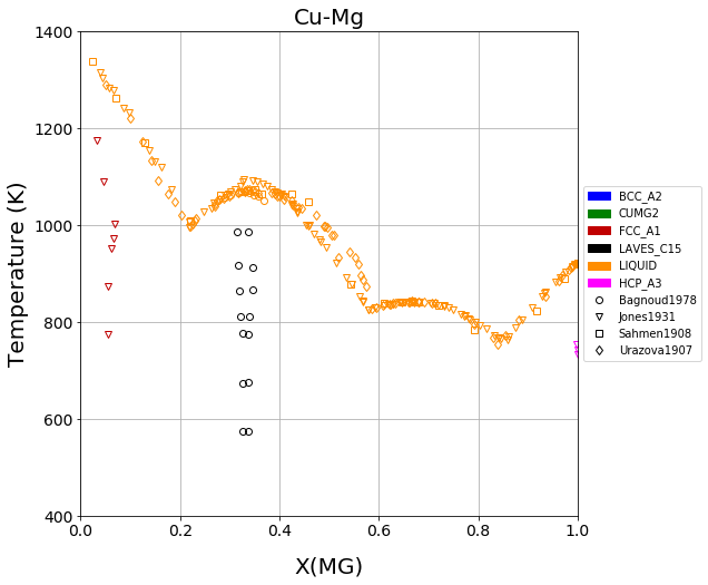
Plotting phaes equilibria data

When compiling ESPEI datasets of phase equilibria data, it can be useful to plot the data to check that it matches visually with what you are expecting. This script plots a binary phase diagram.

TIP: Using this in Jupyter Notebooks make it really fast to update and watch your progress.

"""
This script will create a plot in a couple seconds from a datasets directory
that you can use to check your phase equilibria data.

Change the capitalized variables to the system information and the
directory of datasets you want to plot.
"""

COMPONENTS = ['CU', 'MG', 'VA']
INDEPENDENT_COMPONENT = "MG"  # component to plot on the x-axis
PHASES = ['BCC_A2', 'CUMG2', 'FCC_A1', 'LAVES_C15', 'LIQUID']

DATASETS_DIRECTORY = "~/my-datasets/CU-MG"

X_MIN, X_MAX = 0.0, 1.0
Y_MIN, Y_MAX = 400, 1400

# script starts here, you shouldn't have to edit below this line
import os
from espei.plot import dataplot
from espei.datasets import recursive_glob, load_datasets
from pycalphad import variables as v
import matplotlib.pyplot as plt

plt.figure(figsize=(10,8))

ds = load_datasets(recursive_glob(os.path.expanduser(DATASETS_DIRECTORY), '*.json'))
conds = {v.P: 101325, v.T: (1,1,1), v.X(INDEPENDENT_COMPONENT): (1, 1, 1)}
dataplot(COMPONENTS, PHASES, conds, ds)
plt.xlim(X_MIN, X_MAX)
plt.ylim(Y_MIN, Y_MAX)
plt.show()

The script gives the following output: