Generating Custom Model Parameters

ESPEI’s default parameter selection capabilities support fitting Gibbs energy parameters (G parameters for endmembers, and L parameters for binary and ternary interations) from enthalpy, entropy, and heat capacity data. Using the parameter_generation.fitting_description parameter, ESPEI can support fitting different types of models and data too. For example, the built-in molar volume fitting description can be used to fit molar volume parameters (V0 and VA) to V0 and VM data (see fitting_description in ESPEI YAML input files for more details).

Through these fitting descrptions, ESPEI can be extended to fit custom PyCalphad models and model parameters without changing any of the source code for PyCalphad or ESPEI. Here we will implement a PyCalphad model for BCC elastic stiffness coefficients, which can be uniquly described by three independent components of the elastic stiffness matrix due to the cubic symmetry of the BCC phase. We’ll then use DFT data from [Marker2018] to fit these endmember and interaction parameters and compare the result to values in the original publication. At the end of this tutorial, you will have used ESPEI to generated parameters for three types of elastic constant parameters using DFT data from the literature.

To run ESPEI and generate the output in this tutorial, download the files from here.

Implementing the elastic constant model

Before we can fit parameters to data using ESPEI, we first need a PyCalphad model that can use the parameters. PyCalphad Model objects supports most of the typical Calphad model parameters that are implemented by the commercial Calphad software tools, but here we want to use model parameters that PyCalphad doesn’t have built-in support for. The custom_elastic_model.py file contains the implementation of an ElasticModel class that sublasses the PyCalphad Model class:

import tinydb
from pycalphad import Model
class ElasticModel(Model):
def build_phase(self, dbe):
    phase = dbe.phases[self.phase_name]
    param_search = dbe.search
    for prop in ['C11', 'C12', 'C44']:
        prop_param_query = (
            (tinydb.where('phase_name') == phase.name) & \
            (tinydb.where('parameter_type') == prop) & \
            (tinydb.where('constituent_array').test(self._array_validity))
            )
        prop_val = self.redlich_kister_sum(phase, param_search, prop_param_query).subs(dbe.symbols)
        setattr(self, prop, prop_val)

This class overides the build_phase method of the Model class to add a property to class, one for C11, C12, and C44, where each property is modeled using a Redlich-Kister polynomial, following [Marker2018] Eq. (3). Note that redlich_kister_sum() gives us full generality for an arbitrary number sublattices and species in each sublattice.

Implementing a fitting description

The ElasticModel from the previous section is enough to PyCalphad to use C11, C12, and C44 in a PyCalphad Database object to do calculations and calculate those properties with equilibrium. Now we need to tell ESPEI how to use read datasets for C11, C12, and C44 data, and use this model to fit the corresponding parameters. The two concepts we need are a FittingStep and a ModelFittingDescription.

A FittingStep is an abstract class provided by ESPEI that defines an API for how to fit a particular type of data and what parameters describe it. There’s a 1:1 relationship between a concrete FittingStep and a data type. Fitting steps also have a 1:1 relationship with a parameter type, but note that multiple fitting steps can be used to different data types to a single parameter type. For example, Gibbs energy parameters (G) are fit in three fitting steps: heat capacity data (CPM), then entropy data (SM), then enthalpy data (HM). Below are the implementations for each of the three elastic parameters and data. We are using the AbstractLinearPropertyStep helper class from ESPEI, which is a convience class to make it easier to define FittingStep classes that are 1:1 mappings between a data type and a parameter type and don’t require and linearization or data/model transformation steps.

from espei.parameter_selection.fitting_steps import AbstractLinearPropertyStep

class StepElasticC11(AbstractLinearPropertyStep):
    parameter_name = "C11"
    data_types_read = "C11"

class StepElasticC12(AbstractLinearPropertyStep):
    parameter_name = "C12"
    data_types_read = "C12"

class StepElasticC44(AbstractLinearPropertyStep):
    parameter_name = "C44"
    data_types_read = "C44"

A ModelFittingDescription defines a series of fitting steps that are fit in order, and a PyCalphad model that can use a the parameters to model that data. Here we’ll combine the elastic fitting steps to fit them in order of C11, then C12, then C44. The order of fitting doesn’t matter in this case since the models are independent, but more complex cases might have dependencies requiring certain contributions to be fit before others (e.g. V0 molar volume parameters need to be fit before VA parameters when fitting VM data). By default, ESPEI will use the base PyCalphad Model class, but since that class doesn’t know how to use our custom elastic constant parameters, we need to use the model keyword argument to tell ESPEI to use this model.

from espei.parameter_selection.fitting_descriptions import ModelFittingDescription
elastic_fitting_description = ModelFittingDescription([StepElasticC11, StepElasticC12, StepElasticC44], model=ElasticModel)

The elastic_fitting_description object that we created is the one we will pass to ESPEI via the parameter_generation.fitting_description input parameter.

Defining datasets

Parameter generation can only fit datasets of the same type of non-equilibrium thermochemical data, where the conditions and site fractions to generate the output value are provided explictly. Other than the "output" key that must match one of the data types read by one of our fitting steps, there are no additional steps for ESPEI to be able to read these datasets. See Non-equilibrium Thermochemical Data for a complete description of these type of datasets. Here’s an example for pure BCC Ti from the elastic-datasets directory:

{
    "components": ["TI", "VA"],
    "phases": ["BCC_A2"],
    "output": "C11",
    "values": [[[93]]],
    "conditions": {"T": 298.15, "P": 101325},
    "solver": {"mode": "manual", "sublattice_site_ratios": [1, 3], "sublattice_configurations": [["TI", "VA"]], "sublattice_occupancies": [[1.0, 1.0]]},
    "reference": "Marker (2018)",
    "bibtex": "marker2018binary_elastic",
    "comment": "Values pulled from Table 4 (DFT calculations).",
    "tags": []
}

Running ESPEI

Phase Descriptions defined in phase_model.json are the same as for regular runs of ESPEI:

{
    "components": ["MO", "TI", "ZR", "VA"],
    "phases": {
        "BCC_A2": {
            "sublattice_model": [["MO", "TI", "ZR"], ["VA"]],
            "sublattice_site_ratios": [1, 3]
        }
    }
}

The YAML file that generated parameters for the system described above with the elastic model is in generate_parameters.yaml:

system:
  phase_models: phase_models.json
  datasets: elastic-datasets
generate_parameters:
  excess_model: linear
  ref_state: SGTE91
  fitting_description: custom_elastic_model.elastic_fitting_description
output:
  output_db: Ti-elastic.tdb

The key difference compared to typical runs of ESPEI that fit Gibbs energy parameters is the generate_parameters.fitting_description entry, which is a fully qualified import string to our fitting description object. This is the import path for the object and can be anything that can be imported by the Python interpreter that ESPEI is installed under. In this case, we are importing the object elastic_fitting_description from the custom_elastic_model.py file in the local directory. Note that this can be any local module or an object from any package installed, for example if you have pip installed a package called my_fitting_descriptions that provides a ModelFittingDescrption object for your custom model called my_fit_desc, you would set fitting_description: my_fitting_descriptions.my_fit_desc. If you start a Python interpreter from the same place that you’ll run ESPEI, you can see if ESPEI can detect the fitting description by running the code

from custom_elastic_model import elastic_fitting_description

Finally, we can run this input file using ESPEI by running the command:

espei --in generate_parameters.yaml

That’s it! You should now have a TDB Ti-elastic.tdb that has C11, C22, C44 parameters for pure Ti, Mo, and Zr, and interaction paramters for Ti-Mo and Ti-Zr.

Comparing the results

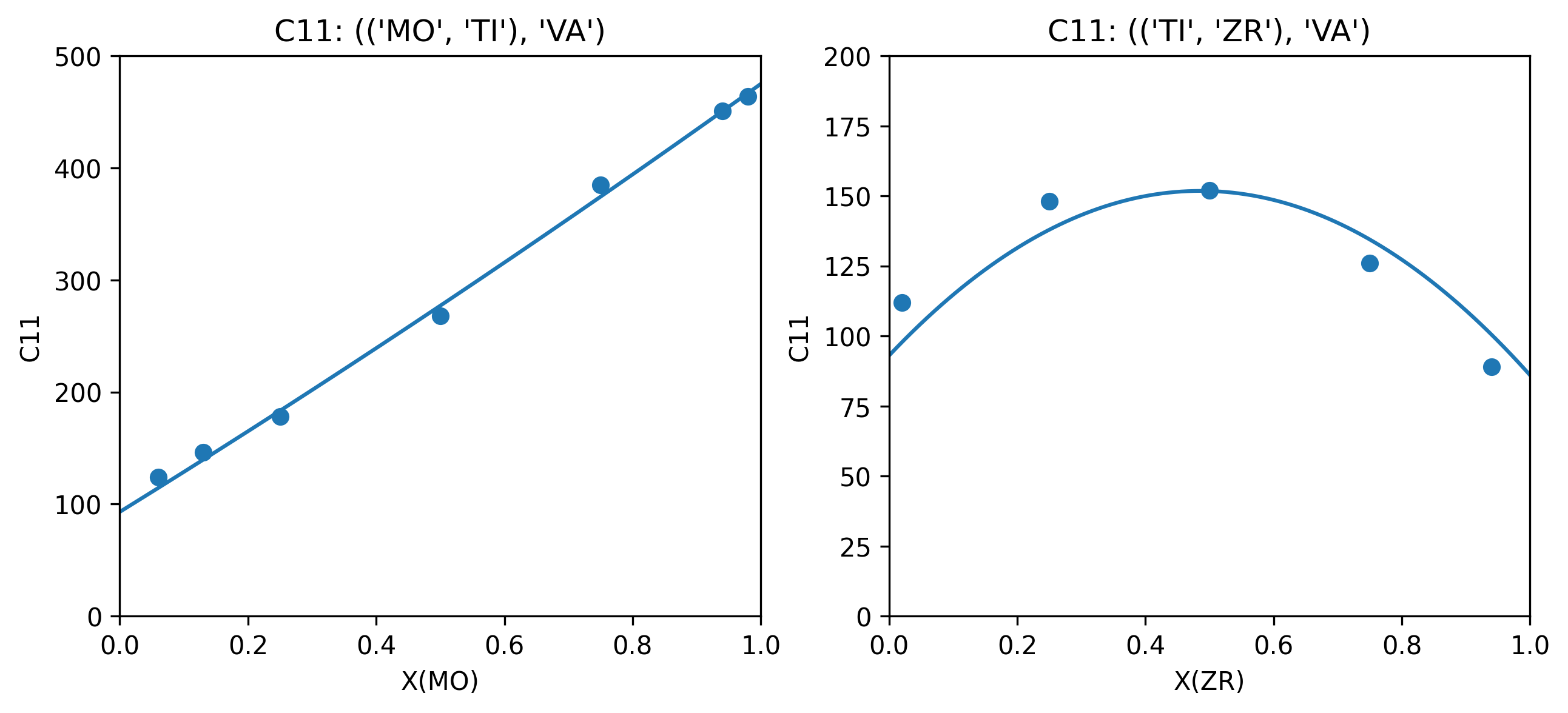
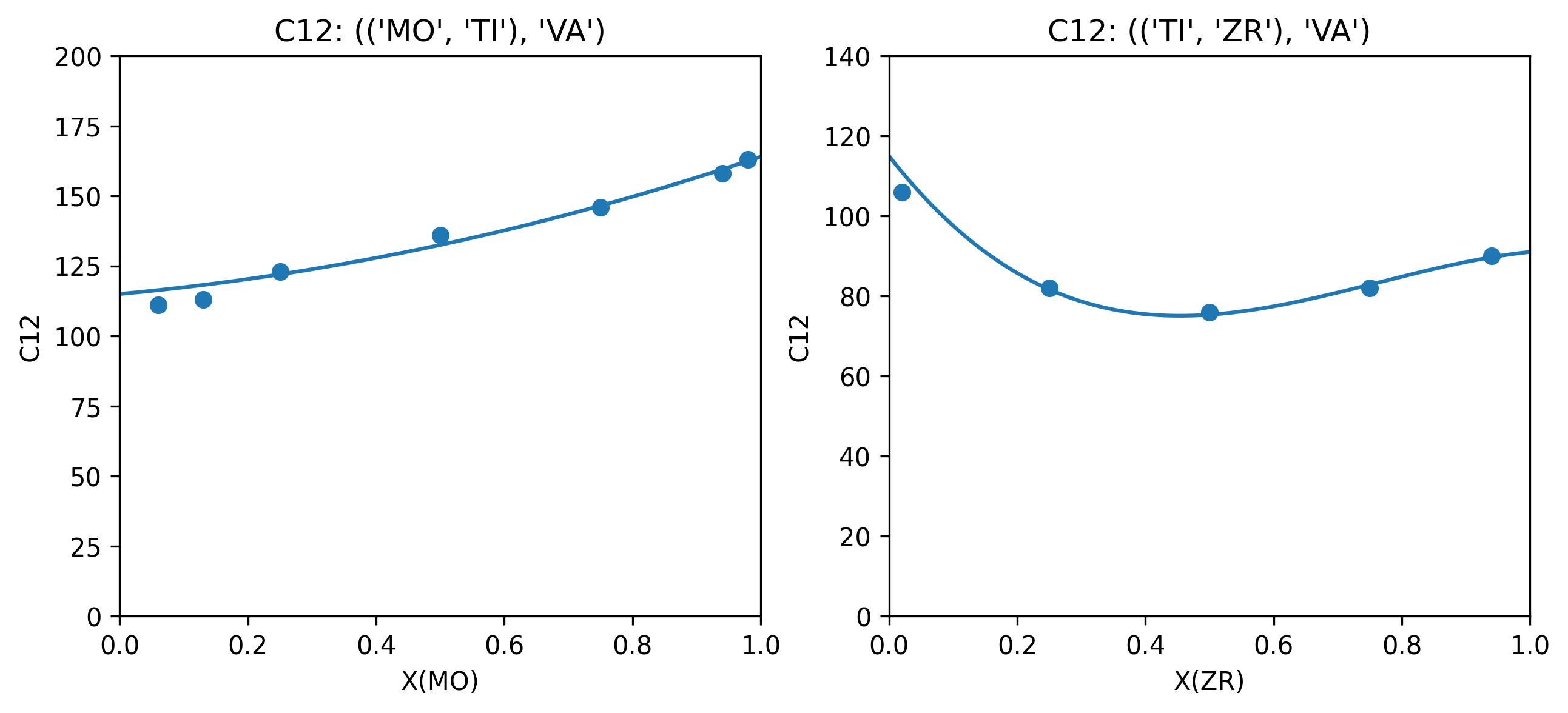
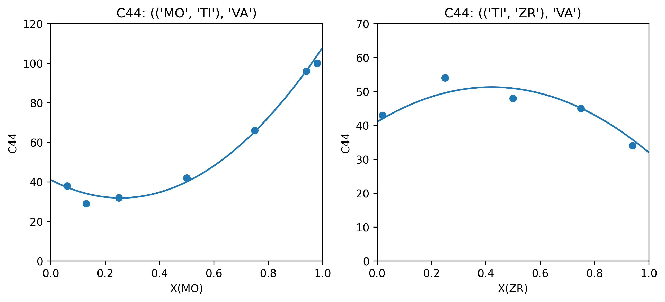
The following table compares the parameters fit by [Marker2018] and those generated by ESPEI. In all cases except for Ti-Zr C11, ESPEI generated the same number of parameters as assessed by Marker et al., where the C11 model is simpler in the version fit by ESPEI. Where the parameters generated are the same, they are close aside from some small differences that could be due to the weighting by Marker et al. (the data used in this tutorial are not weighted). Plots comparing the generated parameters (plotted as lines) in to the data (points) are generated using the plot_model_comparisons.py script and appear to show good agreement.

Param	Interaction	Ti-Mo		Ti-Zr
		Marker (2018)	ESPEI	Marker (2018)	ESPEI
C11	L0	-22.16	-27.7702	246.97	249.001
	L1	0	0	-135.95	0
C12	L0	-36.40	-27.9687	-110.53	-110.725
	L1	0	0	-78.00	-70.2764
C44	L0	-142.9	-137.882	70.06	57.7446
	L1	0	0	0	0