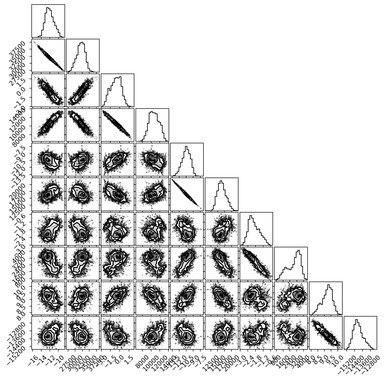
In a corner plot, the distributions for each parameter are plotted along the diagonal and covariances between them under the diagonal. A more circular covariance means that parameters are not correlated to each other, while elongated shapes indicate that the two parameters are correlated.
Strongly correlated parameters are expected for some parameters in Calphad models within phases or for phases in equilibrium, because increasing one parameter while decreasing another would give a similar likelihood.
If you started an MCMC run from scratch, you almost certainly want to discard a number of initial parameters to account for burn-in. The figure produced is relatively small figsize=(8,8) so that it can fit more easily on a page. Larger figures without passing the fig argument to corner.corner will be more legible (try not passing fig to corner.corner).
import matplotlib.pyplot as pltimport numpy as npimport cornertrace = np.load('trace.npy')# the following lines are optional, but useful if your traces are not full# (i.e. your MCMC runs didn't run all their steps)# from espei.analysis import truncate_arrays# lnprob = np.load('lnprob.npy')# trace, lnprob = truncate_arrays(trace, lnprob)burn_in_iterations =500# number of samples of burn-in to discardprint("(# chains, # iterations, # parameters)")print(f"Trace shape: {trace.shape}")print(f"Trace shape after burn-in: {trace[:, burn_in_iterations:, :].shape}")# flatten the along the first dimension containing all the chains in parallelfig = plt.figure(figsize=(8,8)) # figures for corner cannot have axescorner.corner(trace[:, burn_in_iterations:, :].reshape(-1, trace.shape[-1]), fig=fig)fig.show()