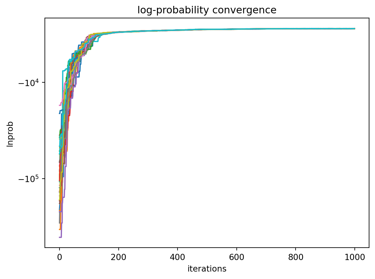
Convergence can be qualitatively estimated by looking at how the log-probability changes for all of the chains as a function of iterations.
Some metrics exist to help estimate convergence, but they should be used with caution, especialy ones that depend on multiple independent chains, as ensemble MCMC methods like the one used by ESPEI do not have independent chains.
Plotting these can also be helpful to estimate how many iterations to discard as burn-in, e.g. in the corner plot example.
import matplotlib.pyplot as pltimport numpy as nplnprob = np.load("lnprob.npy")# the following lines are optional, but useful if your traces are not full# (i.e. your MCMC runs didn't run all their steps)# trace = np.load("trace.npy")# from espei.analysis import truncate_arrays# trace, lnprob = truncate_arrays(trace, lnprob)fig, ax = plt.subplots()ax.plot(lnprob.T)ax.set_title("log-probability convergence")ax.set_xlabel("iterations")ax.set_ylabel("lnprob")ax.set_yscale("symlog") # log-probabilties are often negative, symlog gives log scale for negative numbersfig.show()
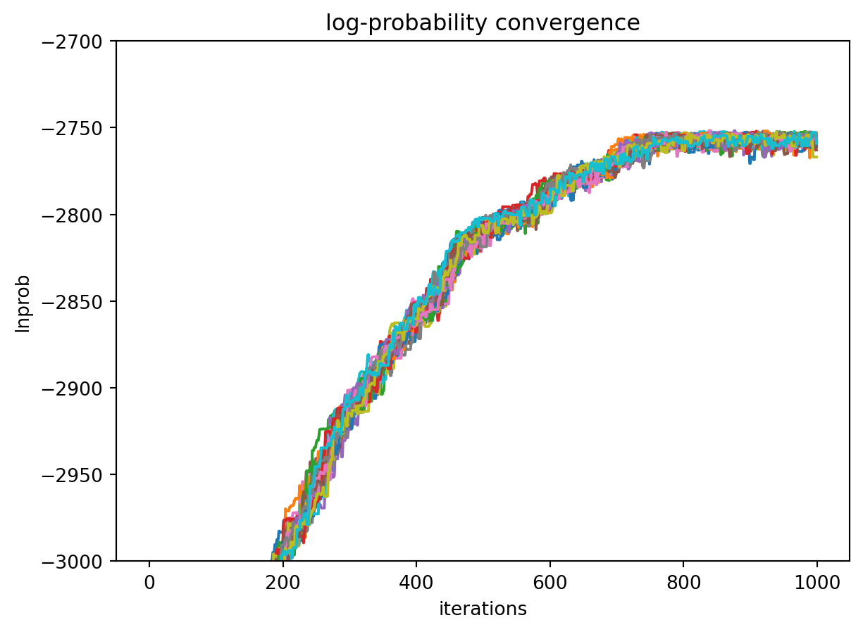
we can zoom in using a linear scale to inspect more closely: