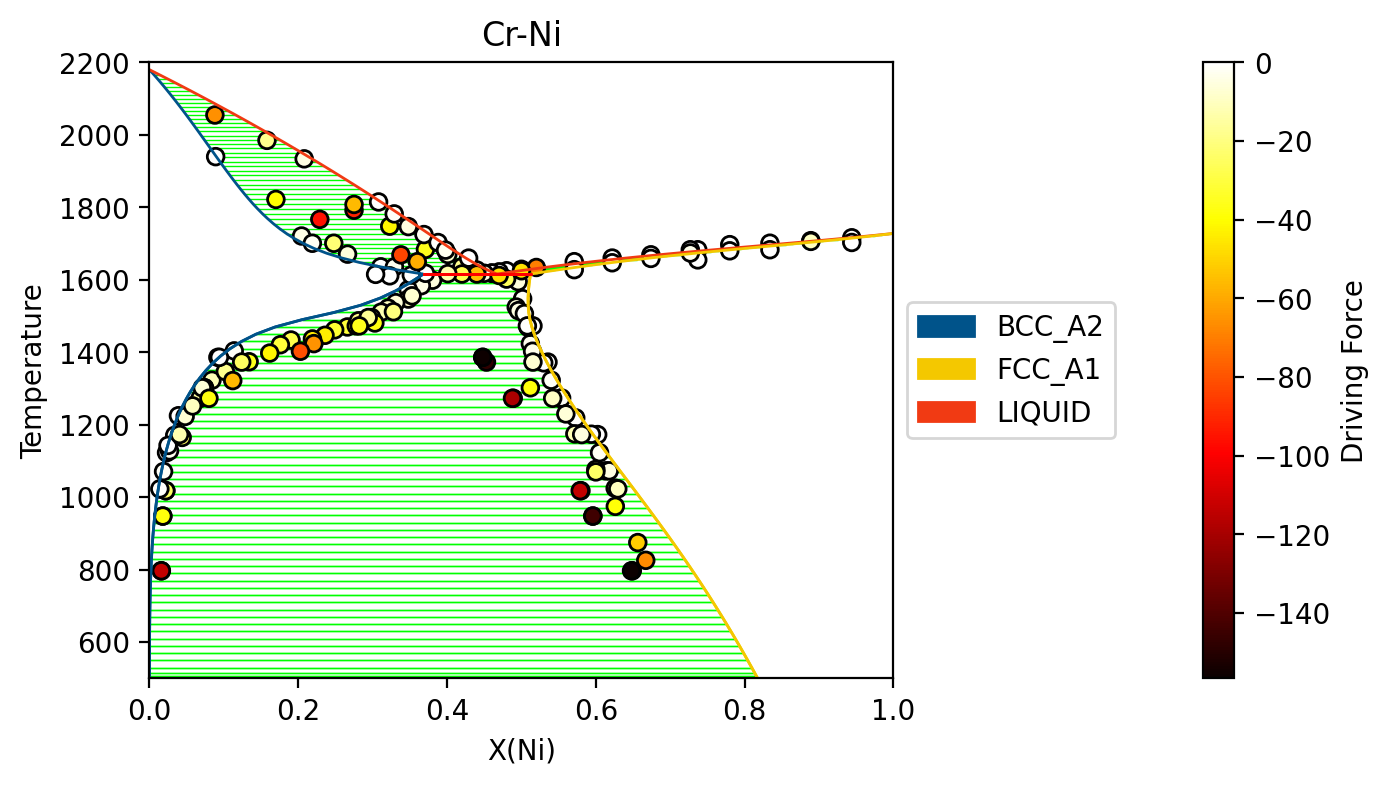
This visualization can be used as a diagnostic for understanding which ZPF data are contributing the most driving force towards the likelihood. Note that these driving forces are unweighted, since the weight is applied when computing the log-likelihood of each driving force.
import numpy as npimport matplotlib.pyplot as pltfrom pycalphad import Database, binplot, variables as vfrom pycalphad.core.utils import extract_parametersfrom espei.datasets import load_datasets, recursive_globfrom espei.error_functions.zpf_error import get_zpf_data, calculate_zpf_driving_forcesdbf = Database("Cr-Ni_mcmc.tdb")comps = ["CR", "NI", "VA"]phases =list(dbf.phases.keys())indep_comp_cond = v.X("NI") # binary assumedconditions = {v.N: 1, v.P: 101325, v.T: (500, 2200, 20), indep_comp_cond: (0, 1, 0.01)}parameters = {} # e.g. {"VV0001": 10000.0}, if empty, will use the current database parameters# Get the datasets, construct ZPF data and compute driving forces# Driving forces and weights are ragged 2D arrays of shape (len(zpf_data), len(vertices in each zpf_data))datasets = load_datasets(recursive_glob("input-data"))zpf_data = get_zpf_data(dbf, comps, phases, datasets, parameters=parameters)param_vec = extract_parameters(parameters)[1]driving_forces, weights = calculate_zpf_driving_forces(zpf_data, param_vec)# Construct the plotting compositions, temperatures and driving forces# Each should have len() == (number of vertices)# Driving forces already have the vertices unrolled so we can concatenate directlyXs = []Ts = []dfs = []for data, data_driving_forces inzip(zpf_data, driving_forces):# zpf_data have (ragged) shape (len(datasets), len(phase_regions), len(vertices))# while driving_forces have (ragged) shape (len(datasets), len(vertices)), concatenating along the phase regions dimension# so we need an offset to account for phase veritices from previous phase regions driving_force_offset =0for phase_region in data["phase_regions"]:for vertex, df inzip(phase_region.vertices, data_driving_forces[driving_force_offset:]): driving_force_offset +=1 comp_cond = vertex.comp_condsif vertex.has_missing_comp_cond:# No composition to plotcontinue dfs.append(df) Ts.append(phase_region.potential_conds[v.T])# Binary assumptions hereassertlen(comp_cond) ==1if indep_comp_cond in comp_cond: Xs.append(comp_cond[indep_comp_cond])else:# Switch the dependent and independent component Xs.append(1.0-tuple(comp_cond.values())[0])# Plot the phase diagram with driving forcesfig, ax = plt.subplots(dpi=100, figsize=(8,4))binplot(dbf, comps, phases, conditions, plot_kwargs=dict(ax=ax), eq_kwargs={"parameters": parameters})sm = plt.cm.ScalarMappable(cmap="hot")sm.set_array(dfs)ax.scatter(Xs, Ts, c=dfs, cmap="hot", edgecolors="k")fig.colorbar(sm, ax=ax, pad=0.25, label="Driving Force")fig.show()